

The wall mostly isn't where the datasheet says
Sweeping an O(n) two-pointer scan from a thousand elements to sixty-four million, across three predicted L1/L2/L3 boundaries, produces a flat cycles-per-element line — not the step function a cache datasheet predicts. The one place a real, sizeable variation shows up is amortized vector growth, and even there it isn't a step: it's a hump that Big-O's own accounting has no vocabulary for.
- A self-manufactured 'memory wall' caught and undone — same mistake as Part 1, hiding on the other end of the size range
- Three predicted cache boundaries (12,288 / 327,680 / 6,291,456 elements) — checked, and absent
- Why a hardware prefetcher protects a two-pointer scan but not a scattered access pattern
- Amortized push_back cycles/push: a hump Big-O's 'amortized O(1)' never promised to explain
Part 1 of this pair ended on a method: loop the algorithm enough times that a cold start stops dominating the measurement, then read cycles off the hardware instead of a clock. That method carried an assumption nobody tested — it was always applied to the same 80-character string, repeated a million times. The input never changed size.
So this piece changes exactly one thing: it sweeps the input itself, from a thousand elements to sixty-four million, and asks the question Part 1 skipped. Big-O says the answer doesn’t matter — O(n) is O(n) whether n is a thousand or a billion, that is the entire point of asymptotic notation. But “cycles per element” is not asymptotic. It is a real, physical number, and physical numbers are exactly the kind of thing that should change once your data stops fitting where the chip expects it to.
It does, and it doesn’t, and getting that wrong the first time is most of what this piece is actually about.
The object: a skyline, and how far apart the two pointers are
The problem this time is LeetCode’s “Container With Most Water”: you’re given a row of vertical walls, one per array index, and asked for the two walls — anywhere in the row — that trap the most water between them. Picture a skyline. Pick two buildings; the water they can hold is the shorter of the two heights, times the distance between them.
The optimal solution is another two-pointer sweep, same shape as Part 1’s sliding window: one pointer at the left end, one at the right, and a rule for which one moves.
class Solution:
    def maxArea(self, height: list[int]) -> int:
        left, right = 0, len(height) - 1
        best = 0

        while left < right:
            h = min(height[left], height[right])
            best = max(best, h * (right - left))

            if height[left] < height[right]:
                left += 1
            else:
                right -= 1

        return best
Move whichever pointer sits at the shorter wall — moving the taller one can only shrink the width without any chance of a taller replacement, so it can never help. Every index gets visited exactly once, by whichever pointer reaches it, so this is O(n): one pass, two runners starting at opposite ends of the array and walking toward each other.

One pass, two runners, opposite ends, same array — the entire reason this problem was chosen over any other O(n) scan. Photo by Nicolas Hoizey on Unsplash.
That “two runners, opposite ends, same array” detail is the whole reason this problem was chosen over any other O(n) scan. It sweeps the entire array on every call, and — unlike Part 1’s fixed 80-character string — the array itself can be any length at all. Which means, for the first time in this series, “how big is the input” is a variable I get to sweep on purpose.
The number: three cache sizes, and what they predict
Part 1 pinned every measurement to CPU core 0 on this machine, a performance core on an Intel i9-12900HK. That core’s cache sizes, read straight from /sys/devices/system/cpu/cpu0/cache/index*/size rather than guessed from a spec sheet:
| Level | Size | ÷ 4 bytes (one C int) |
|---|---|---|
| L1 data | 48 KiB | 12,288 elements |
| L2 | 1,280 KiB | 327,680 elements |
| L3 (shared) | 24,576 KiB | 6,291,456 elements |
Same move as the Neo Geo piece’s bandwidth division: turn a datasheet number into a prediction you can check. If an array’s whole footprint stops fitting in a cache level, the elements that spill out of it have to come from somewhere slower — so the prediction is three step-ups in cycles per element, one at each of those three element counts, as the array grows past 12,288, then 327,680, then 6,291,456 ints.
That prediction is checkable, and — spoiler — mostly wrong, for a reason worth walking through slowly, because I got it wrong myself on the first attempt.
The path: how a load escalates, and how differently three chips build it
A cache size predicts when an access pattern outgrows a level. It says nothing about what happens on the way there. Every load a CPU issues walks the same shaped path — check the closest, smallest store first; on a miss, check the next one out; keep escalating until something answers — but “closest” and “how much farther the next one is” are architecture-specific design choices, not physical constants. The three chips a reader is most likely to be holding right now build that path differently enough that the table above is one implementation of the idea, not the idea itself.
| Level | i9-12900HK, Golden Cove P-core (x86, this piece’s own chip) | Apple M1, Firestorm (ARM, laptop) | Arm Cortex-X4 reference (ARM, phone) |
|---|---|---|---|
| L1 data | 48 KiB, ~5 cycles | 128 KiB, ~3–4 cycles | 64 KiB |
| L2 | 1.25 MiB, private, ~14–15 cycles | 12 MiB, shared by 4 P-cores, ~18 cycles | 0.5–2 MiB, private (configurable) |
| Shared / system cache | 24 MiB L3 — “brutally high” past L2, per Chips and Cheese, once a request crosses the ring bus | 8 MiB SLC, shared with the GPU and neural engine, +10–15 ns past L2 | up to 32 MiB via a DSU; real phones ship closer to 8 MiB |
| DRAM | typically 90–110 ns for this DDR4/DDR5 class | +91 ns past L2 | higher again — LPDDR tuned for power, not latency |
On this piece’s own chip, the path stays short and private for as long as engineering effort can keep it there. Golden Cove’s L1d and L2 are both fast for their size, and the L2 in particular is unusually large for a private, per-core cache — that size is Intel’s answer to a shared L3 whose ring-bus latency it would rather most requests never have to pay.
Apple’s M1 — an ARM core built for a laptop’s power and thermal budget, the closest thing to “ARM desktop” most readers have used — draws the same three-hop shape around different joints. Its L1d is both bigger and faster than the i9’s, a combination that comes from betting a wider core on hit rate over raw clock speed. There is no discrete, per-core L3 at all: four Firestorm performance cores share one L2, and a miss past that lands in a system-level cache — Apple’s name for a cache the CPU shares with the GPU and the neural engine, not just with its own cores — before DRAM.
Shrink the same idea down to a phone and the shape survives the resizing even where neither vendor is involved. Arm’s own Cortex-X4 — the reference design inside the Snapdragon 8 Gen 3, the Dimensity 9300, and Google’s Tensor G4, i.e. most 2024-era Android flagships — publishes its cache sizes as configurable ranges, not fixed numbers, and real phones pick toward the small end of every one of them: commonly around 2 MiB of L2 and 8 MiB of shared cache, against a reference ceiling of 32 MiB, because die area and power on a phone’s thermal budget are scarcer than on the laptop chip sharing half its microarchitecture DNA.

Closest first, escalate on a miss, get slower at every hop out — the shape three vendors agree on even when none of their numbers do. Photo by Tyler on Unsplash.
Three vendors, three sets of numbers, and none of them agree with the i9’s on where a byte should live. What they agree on is the shape: closest first, escalate on a miss, get slower at every hop out. That shared shape is what makes the finding in the next section portable in principle, even though only the i9 got measured here — a hardware prefetcher watching a strictly forward, single-stride access pattern has exactly the same job at every one of these hops, on all three chips, because “the next address is one stride further” is a prediction the escalation path itself never has to get right for the trick to work.
Only the i9 above got measured for this piece, though — so that’s the only chip anything else here can actually vouch for.
The work: a fake memory wall, and how it was manufactured
First pass, done the Part-1 way. Loop the algorithm enough times per size that a cold start doesn’t dominate — but keep the total elements processed roughly constant across sizes, so a small array gets many loops and a huge one gets few. That is exactly the amortization trick from Part 1, applied per size instead of once. Here is what it produced, in C, pinned to core 0:
| n | cycles/element |
|---|---|
| 1,000 | 2.34 |
| 64,000 | 2.23 |
| 1,000,000 | 2.28 |
| 4,000,000 | 2.41 |
| 8,000,000 | 2.63 |
| 32,000,000 | 3.36 |
| 64,000,000 | 4.36 |
That climb past four million elements looks exactly like a memory wall arriving right on schedule — 6,291,456 was the predicted L3 boundary. I believed this number for about ten minutes.
The catch. Building the benchmark array calls rand() once per element — a real, one-time cost, and it scales with n. To keep total elements roughly constant across sizes, the sweep used fewer loop repetitions at large n (eight, for the 64-million case) than at small n. Fewer repetitions means that one-time build cost gets divided by a smaller number — so its contribution to “cycles per element processed” grows exactly where the array is biggest. That is the identical mistake Part 1’s naive single-shot Python run made — a fixed cost, divided by too little repeated work — just hiding on the other end of the size range this time, where doing “more loops per size” runs into “fewer loops at the sizes that need them most.”
Proof, at the single worst offender — n = 64,000,000 — by doing nothing but adding more loop repetitions and watching the number that’s supposed to be a fixed physical property of the hardware move:
| loop repetitions | cycles/element |
|---|---|
| 8 | 4.22 |
| 16 | 3.24 |
| 32 | 2.75 |
| 64 | 2.51 |
| 128 | 2.38 |
| 256 | 2.32 |
That is not a number converging on “memory is slow here.” That is a number converging on 2.3 — the same figure the smallest arrays already showed. The “memory wall” in the first table was the one-time build cost, not the algorithm.
The fix. Hold the loop count constant across every array size instead of holding total elements constant. A fixed build cost, divided by the same number of repetitions every time, contaminates every size point by the same small amount — instead of contaminating the biggest arrays the most. Re-run properly, 500 repetitions at every size, C and C++ side by side:
| n | C, cycles/elem | C++, cycles/elem |
|---|---|---|
| 1,000 | 2.39 | 2.64 |
| 16,000 | 2.32 | 2.45 |
| 64,000 | 2.32 | 2.31 |
| 256,000 | 2.28 | 2.29 |
| 1,000,000 | 2.30 | 2.28 |
| 4,000,000 | 2.32 | 2.32 |
| 16,000,000 | 2.32 | 2.40 |
| 64,000,000 | 2.36 | 2.30 |
Flat. All three predicted cache boundaries — 12,288, 327,680, 6,291,456 — sit inside that table, and none of them show up. std::vector<int> costs nothing over a raw malloc’d array either: same shape, same numbers, within noise.
Why the wall doesn’t arrive. The access pattern is two independent, single-direction reads racing across the array from opposite ends. That is the easiest pattern in the world for a hardware prefetcher: the chip watches each pointer stride forward by one element per step and starts pulling the next cache line in before the loop asks for it — whether that line’s source is L2, L3, or DRAM. Prefetching doesn’t make DRAM as fast as L1; it hides DRAM’s latency behind work the CPU was already going to do. What’s left over, once latency is hidden, is however many instructions the loop body actually needs per element — about fifteen, for this comparison-and-branch loop — and that number doesn’t care where the bytes came from.
Python, same sweep, same fix. Same algorithm, imported straight from the tested Solution class, run over a plain Python list[int] instead of a C array:
| n | Python, cycles/elem |
|---|---|
| 1,000 | 386.08 |
| 16,000 | 404.31 |
| 64,000 | 430.88 |
| 256,000 | 419.73 |
| 1,000,000 | 412.78 |
| 4,000,000 | 431.00 |
| 8,000,000 | 431.46 |
Also flat — just parked about 170 times higher. A Python list is not a row of bytes; it is a row of pointers to individually heap-allocated integer objects, scattered wherever the allocator happened to put them. That ought to be exactly the pattern a prefetcher can’t help with. It doesn’t show up here because the interpreter’s own per-element overhead — dispatching bytecode, looking up __lt__, unboxing two PyLong objects to compare them — is already so much larger than any cache-level latency that there is nothing left for a memory wall to add. Python isn’t immune to the memory hierarchy. It’s just already paying a cost so much bigger that the hierarchy’s cost is a rounding error on top of it.
What “amortized” actually claims, before measuring it
Textbooks define amortized analysis as a way of bounding the total cost of a sequence of operations and dividing that total by the number of operations — not as a probability statement about any single operation, and not an average over random inputs. There is no randomness anywhere in the definition; the bound has to hold for whatever sequence of operations an adversary picks. Cormen, Leiserson, Rivest, and Stein give three ways to derive it. The aggregate method sums the true worst-case cost of every operation in a sequence and divides by the count. The accounting method assigns each operation a fixed amortized charge, lets cheap operations overpay into a credit balance, and lets expensive ones draw that balance down, on the condition that it never goes negative. The potential method formalizes the same credit as a function over the data structure’s state, so an operation’s amortized cost becomes its real cost plus however much it changes that potential. All three are proof techniques for one guarantee: the total cost of any sequence never exceeds the amortized bound times the number of operations in it.
Applied to a doubling dynamic array, the aggregate method is the standard illustration, and it’s worth walking through once because the rest of this section tests exactly this claim. Growing from empty to n elements by repeated doubling triggers a reallocate-and-copy at sizes 1, 2, 4, 8, and so on, up to the largest power of two below n. Those copy costs sum to less than 2n, because a geometric series is bounded by twice its largest term. Divide that total — the copies plus the n pushes themselves — by n operations, and the amortized cost per push is a constant, independent of how large n grows. That derivation is the entire content of the “amortized O(1)” claim std::vector::push_back ships with: a bound on the sum, redistributed evenly across every operation in the proof, whether or not any individual push actually paid that amount.
Small enough to check by hand: sixteen pushes into a doubling array cost 1, 2, 3, 1, 5, 1, 1, 1, 9, then seven more 1s — a copy-and-insert of 1, 2, 4, and 8 elements at pushes 2, 3, 5, and 9, one insert everywhere else. That sums to 31, not 32, and the running average — 1, 1.5, 2, 1.75, 2.4, then a slow settle down to 1.94 by push 16 — never gets far from the bound the proof promises, even though any individual push’s real cost ranges from 1 to 9:
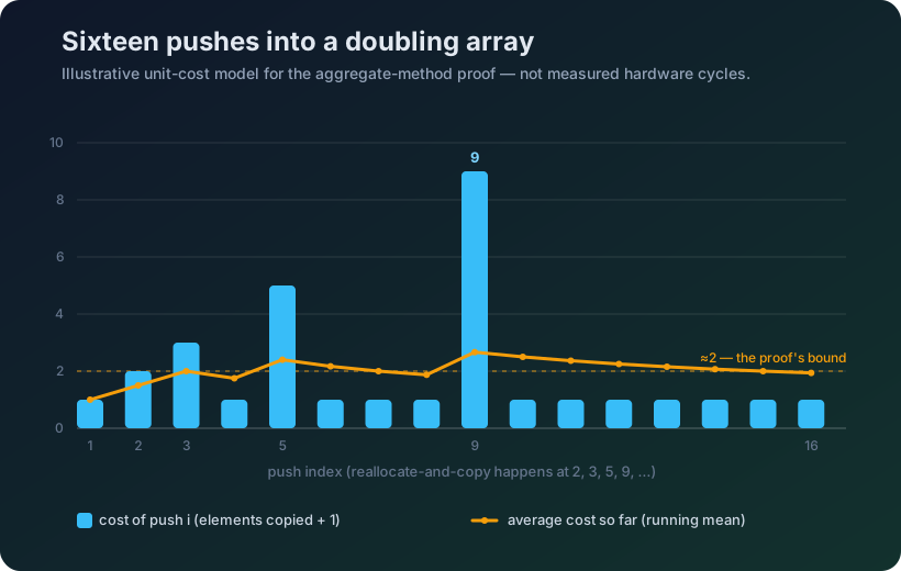
The bars are the aggregate method’s raw material — the true cost of each operation. The line is what “amortized” actually reports back: not any bar’s height, but the running mean across all of them so far, which is the only number the O(1) claim was ever about.
Amortized analysis, with hardware in mind
Every flat table so far measured the easiest access pattern there is. A vector’s growth is a different claim, and the proof above says nothing about whether the copy at any particular size is cheap or expensive on real silicon — only that the sum behaves. That’s checkable the same way every other claim in this piece got checked: grow a vector from empty to size n via push_back, repeatedly, and measure cycles per push.
for (long r = 0; r < repeats; r++) {
  std::vector<int> v;
  for (size_t i = 0; i < n; i++) {
    v.push_back(static_cast<int>(i));
  }
  sum += v.back();
  clobber();  // stop the compiler from proving the loop is dead weight
}
| final size n | cycles/push |
|---|---|
| 1,000 | 1.67 |
| 4,000 | 1.37 |
| 16,000 | 1.38 |
| 64,000 | 3.02 |
| 256,000 | 3.42 |
| 1,000,000 | 3.16 |
| 4,000,000 | 2.81 |
| 16,000,000 | 2.15 |
| 64,000,000 | 2.10 |
Not flat, and not a step function either — it peaks in the middle. The cheapest pushes happen at the smallest and largest sizes tested; the most expensive happen for vectors that finish somewhere between 64,000 and 1,000,000 elements, two and a half times the cost of the cheapest case. “Amortized O(1)” is technically true of every row in that table — the total cost really does divide down to a small constant per push, at every size — and it is also useless for predicting which constant you’ll get, because Big-O’s amortized accounting only ever counted operations. It never asked what any individual operation cost on real silicon, so it has no vocabulary for a curve that goes up and then back down.
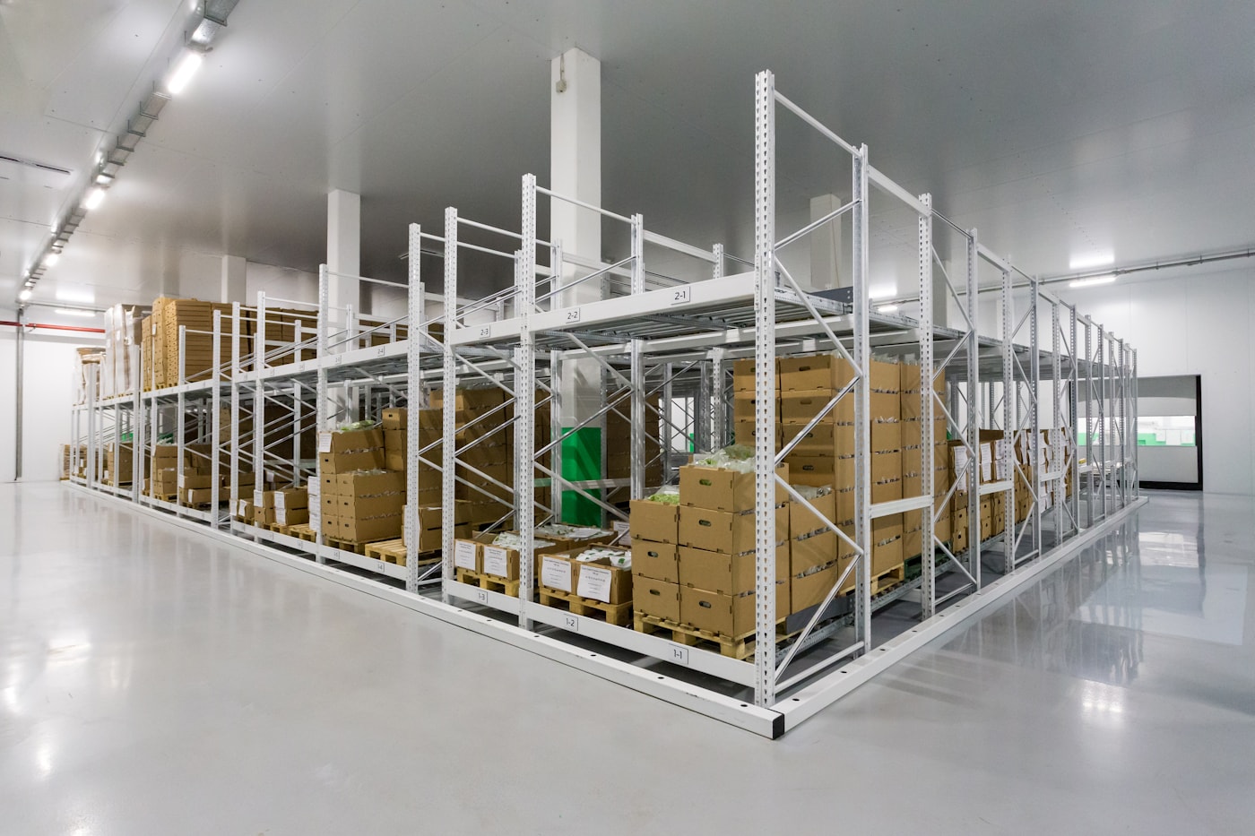
The shelf that has to be rebuilt bigger, unpredictably — the one place in this piece where “amortized constant” and “the same at every size” turned out to be different claims. Photo by Petr on Unsplash.
I don’t have a fully pinned-down cause for the hump, and I’d rather say that plainly than dress up a guess as a finding. The two best candidates are the copy itself crossing a cache boundary the scan never had to (the old and new buffers are both live and both being touched during the copy, doubling the resident footprint the scan never needed to hold at once) and the allocator switching strategy once a single allocation request crosses glibc’s mmap threshold. Telling those apart is a different, smaller experiment than this one — worth doing, not done here.
A number that is “amortized constant” and a number that is “the same at every size” are two different claims, and Big-O only ever promised the first one.
Where this stops being true, and who pays for forgetting
Every flat table above depended on one specific access pattern: two pointers, each moving in only one direction, racing toward each other. A hash-map lookup, a linked structure, or this exact same algorithm fed indices in random order instead of straight from the ends would very likely hit the wall this piece went looking for and didn’t find — prefetching only helps when the next address is predictable, and none of those patterns predict it. The claim here is narrow on purpose: sequential access is protected. Nothing here says scattered access is.
It’s also one core, one chip, one allocator. The vector-growth hump is glibc’s malloc and libstdc++‘s doubling strategy, on this machine, in this kernel; a different allocator, or a vector built with reserve() up front, would tell a different story entirely — probably a much flatter one, since reserve() is precisely the tool that removes the reallocate-and-copy this section measured.
The engineer who pays for skipping this is the one who benchmarks a hot loop against a small, convenient sample — a thousand rows from a test fixture — and ships based on that number, assuming production’s millions of rows scale the same way. For a sequential scan like this one, they’d get lucky: the number really does hold. For anything shaped like the vector-growth case, or anything with a scattered access pattern, they would not — and Big-O’s “still O(n),” true in both cases, gives them no way to tell which one they’re in ahead of time.
Close
None of this changes what to submit to LeetCode, same as Part 1. What changes is smaller: before trusting a “cycles per X” number — even one measured correctly, off real hardware counters — sweep the size of X across a few orders of magnitude first. And when you do, hold your loop count constant across every size instead of your total element count, or you will manufacture a memory wall out of nothing, the same way the first table above did.
Big-O told you the shape of the growth. It was never going to tell you where — or whether — a knee actually sits inside it. Only measuring across sizes does that, and the honest version of the answer, for this problem, on this chip, was: mostly nowhere, and then, in one specific place nobody was asked to look, somewhere unexpected.
References
- LeetCode, Container With Most Water
- Dan Stativa, “Zero Milliseconds Is Not a Score” — Part 1: the perf-over-stopwatch method this piece assumes throughout
- Intel, 12th Gen Intel Core Processors — Performance Hybrid Architecture
- cppreference,
std::vector<T,Allocator>::push_back— amortized-constant complexity, as stated by the standard - Cormen, Leiserson, Rivest, and Stein, Introduction to Algorithms — amortized analysis: the aggregate, accounting, and potential methods, and the doubling-array proof
- Chester Lam (Chips and Cheese), “Popping the Hood on Golden Cove” and “Going Armchair Quarterback on Golden Cove’s Caches” — L1d/L2 latency figures and the L3 ring-bus cost for Golden Cove
- 7-cpu.com, Apple M1 — measured L1/L2/SLC/DRAM latencies in cycles and nanoseconds
- Arm, Cortex-X4 and the Cortex-X4 Core Software Optimization Guide — configurable L1/L2/DSU-shared cache sizes for Arm’s mobile reference design