
Retrieval is an index problem that precedes the model
B-trees, LSM trees, and HNSW are solving the same problem at different scales. This article traces forty years of index engineering into the era of vector search and Kraska's 2018 thesis.
- B-tree and LSM tree mechanics
- Kraska's learned index thesis
- HNSW and ANN search design
- Two-pass retrieval and reranking
- Convergence of storage and GenAI

The first mistake about retrieval is thinking it is search. Search is what a user does. Retrieval is what the system does while the user waits. They look identical from the outside. From the inside, one is a behavior and the other is an index problem that has been evolving for forty years.
Abstract: B-trees and LSM trees are not just data structures. They are explicit bets about when to pay the cost of ordering. Vector indexes make the same bets in high-dimensional space. Kraska’s 2018 insight — that every index is a learned model that stopped learning — is the thread connecting classical storage systems to modern GenAI retrieval. The merge is already underway.
A database index is not a copy of the data. It is a compressed approximation of where the data is.
That word — approximation — matters. It will come back.
1. The Shape of Classical Lookup
Consider a B-tree.
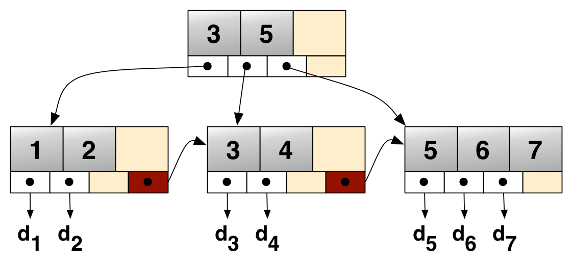
A B-tree is an ordered structure. It assumes the key space is known, discrete, and comparable. It assumes queries will ask: does this key exist, and where does it fit in a sorted sequence?
         [30 | 70]
        /    |    \
   [10|20] [40|60] [80|90]
The B-tree works because the data’s structure mirrors the index. Insert a key, navigate the tree, place it, potentially rebalance. The index stays sorted at all times. This makes point lookups fast and range queries possible.
PostgreSQL, MySQL, SQLite: when you CREATE INDEX, you are almost always building a B-tree. The structural assumption is that query patterns are read-heavy and that the cost of maintaining sorted order is worth paying on every write.
The cost is write amplification. Every insert must navigate, place, and sometimes rebalance.
2. LSM Trees: Deferring the Reckoning
LSM trees — Log-Structured Merge trees — solve a different problem.
They were built for write-heavy workloads. The insight is to accept writes fast and sort later.
write → memtable (sorted, in memory)
                ↓  flush when full
          L0 SSTables (unsorted runs on disk)
                ↓  background compaction
          L1 SSTables (sorted, merged)
                ↓  more compaction
          L2 SSTables (larger, more compact)
The reckoning is deferred. You do not pay the sorting cost at write time. You pay it during compaction — a background process that merges runs into progressively larger, sorted files.
LevelDB, RocksDB, Apache Cassandra: all LSM trees. All designed for situations where writes arrive at a rate that would stall a B-tree under constant rebalancing.
The tradeoff is read amplification. To answer a read, the system may need to check multiple levels. Bloom filters reduce unnecessary disk touches. Block caches reduce repeated reads. But the structural cost of deferred ordering is that reading requires more work.
B-trees pay on write. LSM trees pay on read. Both are conscious bets about when the cost should fall.
Not better and worse. Shaped differently.
3. Kraska 2018: The Model That Was Always There
In 2018, Tim Kraska and colleagues at MIT and Google published The Case for Learned Index Structures.
The paper made one observation that was quiet and structural:
Podcast · O'Reilly Radar · December 2017
How Machine Learning Will Accelerate Data Management Systems
Machine learning will change how we build core algorithms and data structures.Listen to the podcast
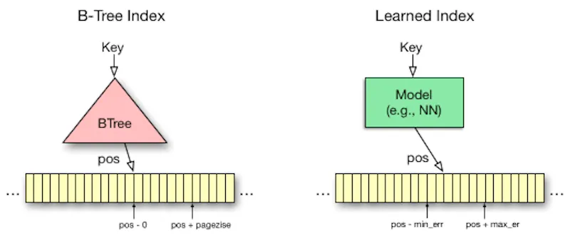
The point is exact: a B-tree does not store the data. It stores a compressed model of the data’s cumulative distribution function — a mapping from key to approximate sorted position.
If a B-tree is already a model, then a trained neural network can be a better model.
They showed this worked. A recursive model index — a small two-stage neural structure — could replace a B-tree index, use significantly less memory, and perform point lookups faster on certain datasets.
This was not a trick. It was a structural observation. The index has always been doing what a model does. It predicts where the data is. B-trees just stopped learning after the initial build.
A B-tree is a static learner. It learns once, from the initial construction, and updates only through inserts and deletes. It does not adapt to shifting query distributions. It does not improve as more data arrives.
A learned index can.
4. What Vectors Are Actually Doing
Vector embeddings solve a structurally different problem from B-tree lookups.
A B-tree answers: where is this exact key?
A vector index answers: what is geometrically close to this point in a high-dimensional space?
classical:  exact(key)  →  sorted position in a known distribution
vector:     embed(text) →  nearest neighbors in ℝ^d
These are not the same kind of question.
Nearest neighbor search in high dimensions is not solved by B-trees. The geometry does not cooperate. Exact nearest neighbor is computationally intractable at scale — the curse of dimensionality means that every point looks roughly equidistant from every other as dimensions increase.
So vector indexes use approximate methods. The two dominant approaches:
IVF (Inverted File Index): partition the embedding space into Voronoi cells during index build. At query time, identify the nearest cell centroids and search only within those cells. The approximation is the bet that the answer is in the nearest cells — a bet that is almost always right and occasionally wrong.
HNSW (Hierarchical Navigable Small World): build a layered graph where each node connects to its approximate nearest neighbors. At query time, navigate the graph greedily from a coarse entry point down through progressively finer layers.
HNSW layers:
  L2:  ○  ─ ─ ─ ─  ○          (sparse, long-range)
  L1:  ○ ─ ○ ─ ○ ─ ○ ─ ○      (medium)
  L0:  ○-○-○-○-○-○-○-○-○-○    (every vector)
Both IVF and HNSW trade exactness for speed. Both make bets about the geometry of the data. Both are, in Kraska’s framing, learned approximations of a distribution — just learned over continuous embedding space rather than discrete key ranges.
The B-tree and HNSW are not as different as they look. Both compress a distribution into a navigable structure. Both answer queries by approximating where the answer should be.
5. Retrieval Is Two Passes
In production GenAI systems, retrieval is almost never one step.
The first pass is fast and approximate. An embedding model converts the query to a vector. ANN search retrieves the top-k candidates from the vector index. The embedding model is coarse — it encodes meaning in aggregate, not in fine-grained relevance. The index is lossy by design. The top-k is deliberately larger than the number you will eventually use.
The second pass is the reranker.
query
  → embed → ANN search → top-100 candidates
                               ↓
                    cross-encoder reranker
                               ↓
                          top-5 results
                               ↓
                        context window
A cross-encoder reranker takes each (query, candidate) pair and scores them jointly. It is slower than ANN search by an order of magnitude. It cannot build an index. But it sees both query and document at the same time, which gives it dramatically better relevance signal than the biencoder used for ANN.
The biencoder is fast because it separates encoding: embed the document once at index time, embed the query at runtime, compare vectors. The cross-encoder is accurate because it does not separate: it attends across the concatenated pair.
The engineering rule is the same as threads and processes: use the fast structure for the broad filter, the accurate structure for the final selection. Do not run the expensive tool on the full set.
6. The Convergence
Here is the question Kraska’s paper opens without fully closing.
If a B-tree is already a learned model, and a vector index is explicitly a learned structure, and a reranker is a neural model — what is the actual boundary between a database and a GenAI system?
Look at what is already running in production:
- pgvector: vector indexes living inside PostgreSQL next to B-tree indexes on the same table, in the same transaction
- Hybrid search: BM25 inverted indexes combined with dense vector search in Elasticsearch, Vespa, and Weaviate — classical term matching and semantic similarity as joint signals
- SPLADE: a language model produces learned sparse vectors — term weights that a classical inverted index can store, but a transformer computed
- ColBERT: per-token embeddings with MaxSim aggregation, borrowing the inverted index structure to store token-level representations at scale
These are not research curiosities. They run in products that handle millions of queries.
The direction is clear.
Classical storage systems are acquiring the properties of learned models: adaptive indexing, learned query planners, ML-guided compaction in LSM trees. GenAI retrieval systems are borrowing from classical index design: inverted files, hybrid ranking, approximate partitioning.
The B-tree does not die. It becomes one layer in a deeper structure that also learns.
The LSM tree does not die. Its compaction logic — iteratively reorganizing data under pressure to minimize future read cost — begins to resemble gradient descent.
7. What This Means for Builders
If you are building retrieval for AI products today, this convergence has concrete consequences.
The embedding model is the implicit index structure. Changing the embedding model changes the geometry of the space. Changing the geometry makes the existing index stale. A reindex is not optional — it is the equivalent of rebuilding a B-tree after changing the sort key. This is not always communicated to the people who own the infra budget.
Retrieval is not a commodity step. Choosing between exact keyword search, approximate vector search, hybrid ranking, and learned sparse retrieval is a structural decision about what kind of approximation you are willing to accept — and under which query distribution. There is no universally correct answer.
Reranking is where Kraska’s critique lands hardest. A reranker is a model that has learned to predict relevance. It reflects the distribution of its training data. A reranker trained on one domain may be confidently wrong in another. The same critique Kraska made of static B-trees applies to static rerankers: they do not adapt to shifting distributions. The relevance function is a bet on future queries matching past queries.
The honest engineering discipline is the same as it was for B-trees, for LSM trees, for threads and processes:
understand the shape of the problem
before choosing the structure
Do not ask which retrieval tool is best. Ask which approximation fits the distribution you actually have.
8. Closing
Classical storage systems and GenAI retrieval are not converging by coincidence.
They were always solving the same underlying problem: how to find something relevant in a large space, quickly, without being certain it exists.
B-trees did it with ordered assumptions. LSM trees did it by deferring the sorting cost. HNSW does it with navigable graph approximation. Rerankers do it with learned relevance.
Kraska’s insight was not that models would replace indexes. It was that indexes were already models — just ones that stopped learning after the build.
The question for the next decade is not whether AI systems will use databases. They already do. The question is what happens when the index learns continuously, the query planner trains on usage, and the relevance function is a weight matrix rather than a hand-written rule.
What it becomes is not a database in the classical sense.
But it is not a model in the classical sense either.
It is something running right now, on every server that answers a question, that we do not yet have a clean word for.